Microstructure analysis

This example shows how you can use PyAdditive to determine the microstructure for a sample coupon with given material and machine parameters.

Units are SI (m, kg, s, K) unless otherwise noted.

Perform required import and connect

Perform the required import and connect to the Additive service.

from ansys.additive.core import Additive, AdditiveMachine, MicrostructureInput, SimulationError

additive = Additive()

user data path: /home/runner/.local/share/pyadditive

Select material

Select a material. You can use the materials_list() method to obtain a list of available materials.

print("Available material names: {}".format(additive.materials_list()))

Available material names: ['316L', 'Ti64', '17-4PH', 'CoCr', 'IN718', 'IN625', 'AlSi10Mg', 'Al357']

You can obtain the parameters for a single material by passing a name from the materials list to the material() method.

material = additive.material("17-4PH")

Specify machine parameters

Specify machine parameters by first creating an AdditiveMachine object and then assigning the desired values. All values are in SI units (m, kg, s, K) unless otherwise noted.

machine = AdditiveMachine()

# Show available parameters
print(machine)

AdditiveMachine
laser_power: 195 W
scan_speed: 1.0 m/s
heater_temperature: 80 °C
layer_thickness: 5e-05 m
beam_diameter: 0.0001 m
starting_layer_angle: 57 °
layer_rotation_angle: 67 °
hatch_spacing: 0.0001 m
slicing_stripe_width: 0.01 m

Set laser power and scan speed

Set the laser power and scan speed.

machine.scan_speed = 1  # m/s
machine.laser_power = 500  # W

Specify inputs for microstructure simulation

Microstructure simulation inputs can include thermal parameters. Thermal parameters consist of cooling_rate, thermal_gradient, melt_pool_width, and melt_pool_depth. If thermal parameters are not specified, the thermal solver is used to obtain the parameters prior to running the microstructure solver.

# Specify microstructure inputs with thermal parameters
input_with_thermal = MicrostructureInput(
    machine=machine,
    material=material,
    id="micro-with-thermal",
    sensor_dimension=0.0005,
    sample_size_x=0.001,  # in meters (1 mm), must be >= sensor_dimension + 0.0005
    sample_size_y=0.001,  # in meters (1 mm), must be >= sensor_dimension + 0.0005
    sample_size_z=0.0015,  # in meters (1 mm), must be >= sensor_dimension + 0.001
    use_provided_thermal_parameters=True,
    cooling_rate=1.1e6,  # °K/s
    thermal_gradient=1.2e7,  # °K/m
    melt_pool_width=1.5e-4,  # meters (150 microns)
    melt_pool_depth=1.1e-4,  # meters (110 microns)
)

# Specify microstructure inputs without thermal parameters
input_without_thermal = MicrostructureInput(
    machine=machine,
    material=material,
    id="micro-without-thermal",
    sensor_dimension=0.0005,
    sample_size_x=0.001,  # in meters (1 mm), must be >= sensor_dimension + 0.0005
    sample_size_y=0.001,  # in meters (1 mm), must be >= sensor_dimension + 0.0005
    sample_size_z=0.0015,  # in meters (1 mm), must be >= sensor_dimension + 0.001
    # use_provided_thermal_parameters defaults to False
)

Run simulation

Use the simulate() method of the additive object to run the simulation. The returned object is either a MicrostructureSummary object or a SimulationError object.

summary = additive.simulate(input_with_thermal)
if isinstance(summary, SimulationError):
    raise Exception(summary.message)

Single input

Plot results

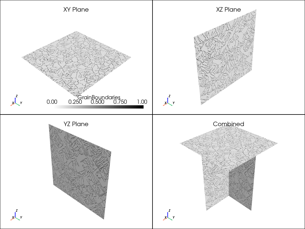
The summary` object includes three VTK files, one for each of the XY, XZ, and YZ planes. Each VTK file contains data sets for grain orientation, boundaries, and number. In addition, the summary object includes circle equivalence data and average grain size for each plane. See MicrostructureSummary for details.

from matplotlib import colors
from matplotlib.colors import LinearSegmentedColormap as colorMap
import matplotlib.pyplot as plt
from matplotlib.ticker import PercentFormatter
import pandas as pd
import pyvista as pv

from ansys.additive.core import CircleEquivalenceColumnNames

Plot 2D grain visualizations

Plot the planar data, read VTK data in data set objects, and create a color map to use with the boundary map.

# Function to plot the planar data
def plot_microstructure(
    xy_data: any, xz_data: any, yz_data: any, scalars: str, cmap: colors.LinearSegmentedColormap
):
    """Convenience function to plot microstructure VTK data."""
    font_size = 8
    plotter = pv.Plotter(shape=(2, 2), lighting="three lights")
    plotter.show_axes_all()
    plotter.add_mesh(xy_data, cmap=cmap, scalars=scalars)
    plotter.add_title("XY Plane", font_size=font_size)

    plotter.subplot(0, 1)
    plotter.add_mesh(xz_data, cmap=cmap, scalars=scalars)
    plotter.add_title("XZ Plane", font_size=font_size)

    plotter.subplot(1, 0)
    plotter.add_mesh(yz_data, cmap=cmap, scalars=scalars)
    plotter.add_title("YZ Plane", font_size=font_size)

    plotter.subplot(1, 1)
    plotter.add_mesh(xy_data, cmap=cmap, scalars=scalars)
    plotter.add_mesh(xz_data, cmap=cmap, scalars=scalars)
    plotter.add_mesh(yz_data, cmap=cmap, scalars=scalars)
    plotter.add_title("Combined", font_size=font_size)

    return plotter


# Read VTK data into pyvista.DataSet objects
xy = pv.read(summary.xy_vtk)
xz = pv.read(summary.xz_vtk)
yz = pv.read(summary.yz_vtk)

# Create a color map to use with the boundary plot
white_black_cmap = colorMap.from_list("whiteblack", ["white", "black"])

plot_microstructure(xy, xz, yz, "GrainBoundaries", white_black_cmap).show(title="Grain Boundaries")
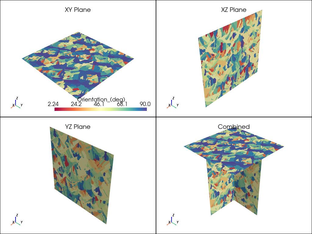
plot_microstructure(xy, xz, yz, "Orientation_(deg)", "spectral").show(title="Orientation °")
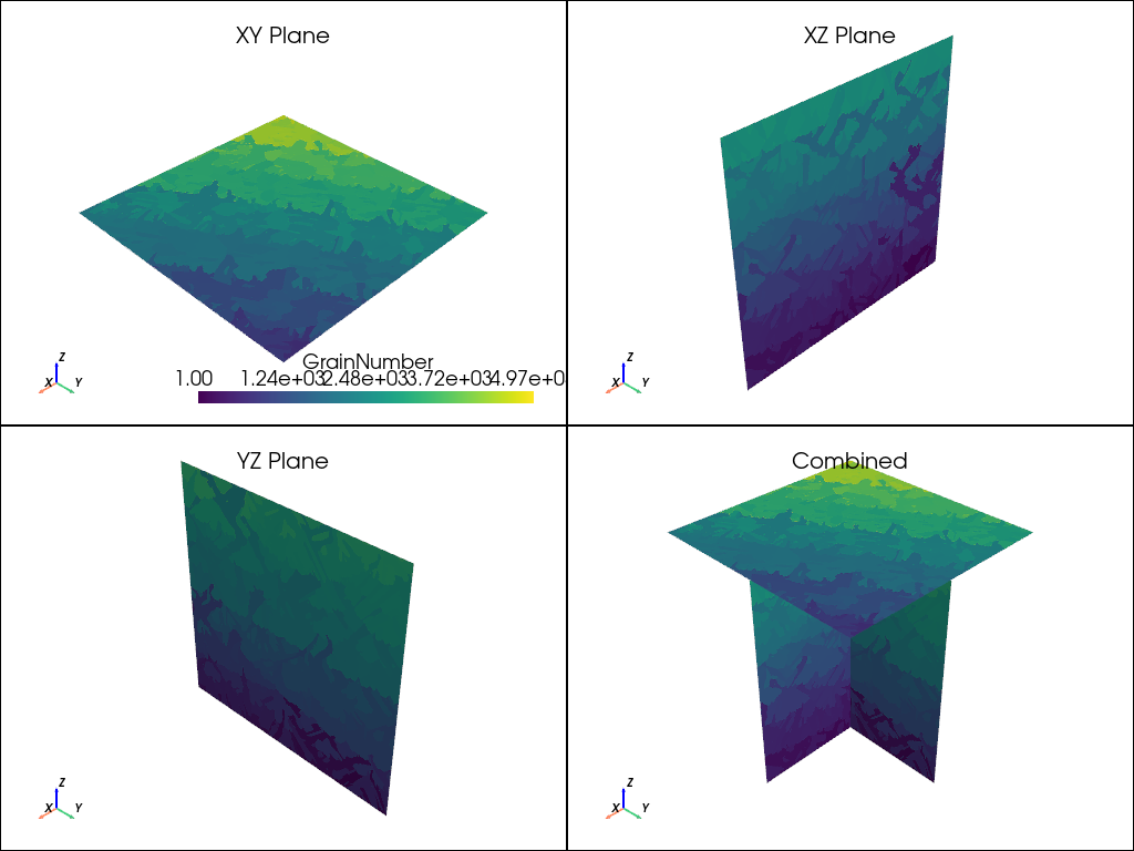
plot_microstructure(xy, xz, yz, "GrainNumber", None).show(title="Grain Number")

• 
• 
• 

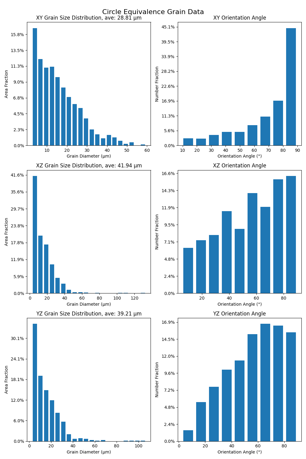
Plot grain statistics

Add grain statistic plots to a figure, create a figure for grain statistics, and then plot the figure.

# Function to simplify plotting grain statistics
def add_grain_statistics_to_figure(
    plane_data: pd.DataFrame,
    plane_str: str,
    plane_ave_grain_size: float,
    diameter_axes: plt.Axes,
    orientation_axes: plt.Axes,
):
    """Convenience function to add grain statistic plots to a figure."""
    xmax = len(plane_data[CircleEquivalenceColumnNames.DIAMETER])
    diameter_axes.hist(plane_data[CircleEquivalenceColumnNames.DIAMETER], bins=20, rwidth=0.75)
    diameter_axes.set_xlabel(f"Grain Diameter (µm)")
    diameter_axes.set_ylabel("Area Fraction")
    diameter_axes.set_title(
        plane_str.upper() + f" Grain Size Distribution, ave: {plane_ave_grain_size:.2f} µm"
    )
    diameter_axes.yaxis.set_major_formatter(PercentFormatter(xmax=xmax))
    orientation_axes.hist(
        plane_data[CircleEquivalenceColumnNames.ORIENTATION_ANGLE], bins=9, rwidth=0.75
    )
    orientation_axes.yaxis.set_major_formatter(PercentFormatter(xmax=xmax))
    orientation_axes.set_xlabel(f"Orientation Angle (°)")
    orientation_axes.set_ylabel("Number Fraction")
    orientation_axes.set_title(plane_str.upper() + " Orientation Angle")


# Create figure for grain statistics
fig, axs = plt.subplots(3, 2, figsize=(10, 15), tight_layout=True)
fig.suptitle("Circle Equivalence Grain Data", fontsize=16)
add_grain_statistics_to_figure(
    summary.xy_circle_equivalence, "xy", summary.xy_average_grain_size, axs[0][0], axs[0][1]
)
add_grain_statistics_to_figure(
    summary.xz_circle_equivalence, "xz", summary.xz_average_grain_size, axs[1][0], axs[1][1]
)
add_grain_statistics_to_figure(
    summary.yz_circle_equivalence, "yz", summary.yz_average_grain_size, axs[2][0], axs[2][1]
)
plt.show()