Note
Go to the end to download the full example code.
Single bead analysis#
This example shows how to use PyAdditive to determine melt pool characteristics for a given material and machine parameter combinations.
Units are SI (m, kg, s, K) unless otherwise noted.
Perform required imports and connect#
Perform the required imports and connect to the Additive service.
import os

import matplotlib.pyplot as plt
import pyvista as pv

from ansys.additive.core import (
    Additive,
    AdditiveMachine,
    MeltPoolColumnNames,
    SimulationError,
    SingleBeadInput,
)

additive = Additive()
Get server connection information#
Get server connection information using the about() method.
print(additive.about())
ansys.additive.core version 0.20.0
Client side API version: 5.0.3
Server localhost:50052 is connected.
  API version: 5.0.3
  Version: 25.2.1
Select material#
Select a material. You can use the materials_list() method to
obtain a list of available materials.
print("Available material names: {}".format(additive.materials_list()))
Available material names: ['IN718', '17-4PH', 'Al357', 'Ti64', 'CoCr', '316L', 'IN625', 'AlSi10Mg']
You can obtain the parameters for a single material by passing a name
from the materials list to the material() method.
material = additive.material("IN718")
Specify machine parameters#
Specify machine parameters by first creating an AdditiveMachine object
and then assigning the desired values. All values are in SI units (m, kg, s, K)
unless otherwise noted.
machine = AdditiveMachine()

# Show available parameters
print(machine)
AdditiveMachine
laser_power: 195 W
scan_speed: 1.0 m/s
heater_temperature: 80 °C
layer_thickness: 5e-05 m
beam_diameter: 0.0001 m
starting_layer_angle: 57 °
layer_rotation_angle: 67 °
hatch_spacing: 0.0001 m
slicing_stripe_width: 0.01 m
Set laser power and scan speed#
Set the laser power and scan speed.
machine.scan_speed = 1  # m/s
machine.laser_power = 300  # W
Specify inputs for single bead simulation#
Create a SingleBeadInput object containing the desired simulation parameters.
input = SingleBeadInput(
    machine=machine,
    material=material,
    bead_length=0.0012,  # meters
    output_thermal_history=True,
    thermal_history_interval=1,
)
Run simulation#
Use the simulate() method of the additive object to run the simulation.
The returned object is either a SingleBeadSummary object containing the input
and a MeltPool or a SimulationError object.
summary = additive.simulate(input)
if isinstance(summary, SimulationError):
    raise Exception(summary.message)
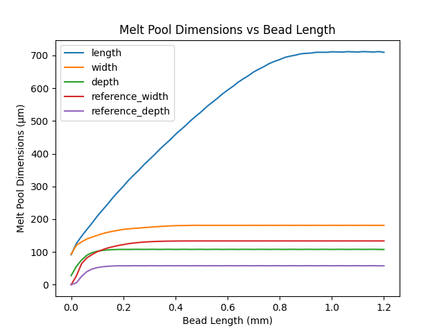
Plot melt pool statistics#
Obtain a Pandas DataFrame instance containing the melt pool
statistics by using the data_frame() method of the melt_pool
attribute of the summary object. The column names for the DataFrame
instance are described in the documentation for data_frame(). Use the
plot() method to plot the melt pool dimensions as a function
of bead length.
df = summary.melt_pool.data_frame().multiply(1e6)  # convert from meters to microns
df.index *= 1e3  # convert bead length from meters to millimeters

df.plot(
    y=[
        MeltPoolColumnNames.LENGTH,
        MeltPoolColumnNames.WIDTH,
        MeltPoolColumnNames.DEPTH,
        MeltPoolColumnNames.REFERENCE_WIDTH,
        MeltPoolColumnNames.REFERENCE_DEPTH,
    ],
    ylabel="Melt Pool Dimensions (µm)",
    xlabel="Bead Length (mm)",
    title="Melt Pool Dimensions vs Bead Length",
)
plt.show()
List melt pool statistics#
You can show a table of the melt pool statistics by typing the name of the
data frame object and pressing enter. For brevity, the following code
uses the head() method so that only the first few rows are shown.
Note, if running this example as a Python script, no output is shown.
df.head()
Save melt pool statistics#
Save the melt pool statistics to a CSV file using the
to_csv() method.
df.to_csv("melt_pool.csv")
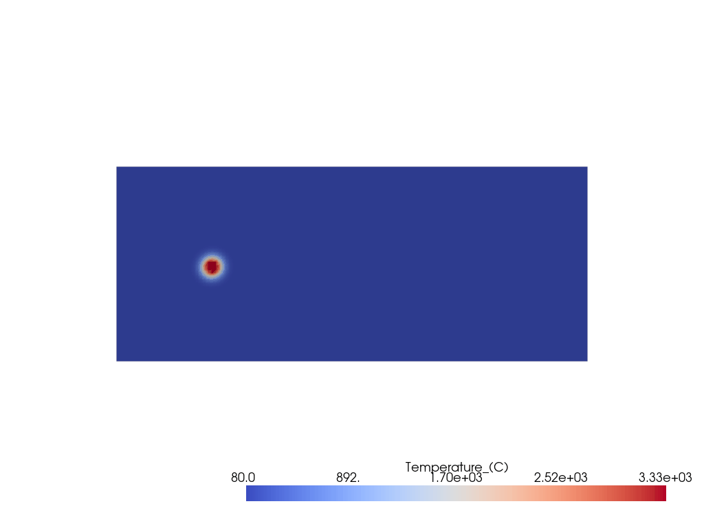
Plot thermal history#
Plot the thermal history of the single bead simulation using the class
pyvista.Plotter. The plot shows the temperature
distribution in the melt pool at each time step.
plotter_xy = pv.Plotter(notebook=False, off_screen=True)
plotter_xy.open_gif("thermal_history_xy.gif")

path = summary.melt_pool.thermal_history_output
files = [f for f in os.listdir(path) if f.endswith(".vtk")]

for i in range(len(files)):
    i = f"{i:07}"
    mesh = pv.read(os.path.join(path, f"GridFullThermal_L0000000_T{i}.vtk"))
    plotter_xy.add_mesh(mesh, scalars="Temperature_(C)", cmap="coolwarm")
    plotter_xy.view_xy()
    plotter_xy.write_frame()

plotter_xy.close()
Print the simulation logs#
To print the simulation logs, use the logs() property.
print(summary.logs)
File: thermal-log.log
Thu May 29 21:37:32 2025 -> SOLVERINFO: Number of elements traveled by laser per step: 1.333333
Thu May 29 21:37:34 2025 -> DESKTOPINFO: License successfully obtained.
Thu May 29 21:37:34 2025 -> SOLVERINFO: Skipping HPC license checkout as 4 are being requested.
Thu May 29 21:37:34 2025 -> USERINFO: Starting ThermalSolver v33.2.5, SolverCommon v14.108.0
Thu May 29 21:37:34 2025 -> SOLVERINFO: Begin Run
Thu May 29 21:37:34 2025 -> DESKTOPINFO: Using 4 threads for solver
Thu May 29 21:37:38 2025 -> SOLVERINFO: Lost power from capping: 0.000000W over 0 Nodes. Ratio to input power: 0.000000
Thu May 29 21:37:38 2025 -> SOLVERINFO: PercentComplete: 1.64
Thu May 29 21:37:38 2025 -> SOLVERINFO: Lost power from capping: 5.737448W over 10 Nodes. Ratio to input power: 0.032991
Thu May 29 21:37:38 2025 -> SOLVERINFO: PercentComplete: 3.28
Thu May 29 21:37:38 2025 -> SOLVERINFO: Lost power from capping: 12.812348W over 30 Nodes. Ratio to input power: 0.073672
Thu May 29 21:37:38 2025 -> SOLVERINFO: PercentComplete: 4.92
Thu May 29 21:37:38 2025 -> SOLVERINFO: Lost power from capping: 21.200940W over 42 Nodes. Ratio to input power: 0.121907
Thu May 29 21:37:39 2025 -> SOLVERINFO: PercentComplete: 6.56
Thu May 29 21:37:39 2025 -> SOLVERINFO: Lost power from capping: 25.335262W over 51 Nodes. Ratio to input power: 0.145680
Thu May 29 21:37:39 2025 -> SOLVERINFO: PercentComplete: 8.2
Thu May 29 21:37:39 2025 -> SOLVERINFO: Lost power from capping: 27.828174W over 56 Nodes. Ratio to input power: 0.160014
Thu May 29 21:37:39 2025 -> SOLVERINFO: PercentComplete: 9.84
Thu May 29 21:37:39 2025 -> SOLVERINFO: Lost power from capping: 28.831713W over 60 Nodes. Ratio to input power: 0.165785
Thu May 29 21:37:40 2025 -> SOLVERINFO: PercentComplete: 11.5
Thu May 29 21:37:40 2025 -> SOLVERINFO: Lost power from capping: 29.521726W over 63 Nodes. Ratio to input power: 0.169752
Thu May 29 21:37:40 2025 -> SOLVERINFO: PercentComplete: 13.1
Thu May 29 21:37:40 2025 -> SOLVERINFO: Lost power from capping: 29.950405W over 66 Nodes. Ratio to input power: 0.172217
Thu May 29 21:37:40 2025 -> SOLVERINFO: PercentComplete: 14.8
Thu May 29 21:37:40 2025 -> SOLVERINFO: Lost power from capping: 29.885058W over 65 Nodes. Ratio to input power: 0.171842
Thu May 29 21:37:41 2025 -> SOLVERINFO: PercentComplete: 16.4
Thu May 29 21:37:41 2025 -> SOLVERINFO: Lost power from capping: 30.008476W over 66 Nodes. Ratio to input power: 0.172551
Thu May 29 21:37:41 2025 -> SOLVERINFO: PercentComplete: 18
Thu May 29 21:37:41 2025 -> SOLVERINFO: Lost power from capping: 30.208566W over 67 Nodes. Ratio to input power: 0.173702
Thu May 29 21:37:41 2025 -> SOLVERINFO: PercentComplete: 19.7
Thu May 29 21:37:41 2025 -> SOLVERINFO: Lost power from capping: 30.007352W over 67 Nodes. Ratio to input power: 0.172545
Thu May 29 21:37:42 2025 -> SOLVERINFO: PercentComplete: 21.3
Thu May 29 21:37:42 2025 -> SOLVERINFO: Lost power from capping: 30.066847W over 67 Nodes. Ratio to input power: 0.172887
Thu May 29 21:37:42 2025 -> SOLVERINFO: PercentComplete: 23
Thu May 29 21:37:42 2025 -> SOLVERINFO: Lost power from capping: 30.238380W over 67 Nodes. Ratio to input power: 0.173873
Thu May 29 21:37:42 2025 -> SOLVERINFO: PercentComplete: 24.6
Thu May 29 21:37:42 2025 -> SOLVERINFO: Lost power from capping: 30.022184W over 67 Nodes. Ratio to input power: 0.172630
Thu May 29 21:37:43 2025 -> SOLVERINFO: PercentComplete: 26.2
Thu May 29 21:37:43 2025 -> SOLVERINFO: Lost power from capping: 30.074410W over 67 Nodes. Ratio to input power: 0.172930
Thu May 29 21:37:43 2025 -> SOLVERINFO: PercentComplete: 27.9
Thu May 29 21:37:43 2025 -> SOLVERINFO: Lost power from capping: 30.241876W over 67 Nodes. Ratio to input power: 0.173893
Thu May 29 21:37:43 2025 -> SOLVERINFO: PercentComplete: 29.5
Thu May 29 21:37:43 2025 -> SOLVERINFO: Lost power from capping: 30.023920W over 67 Nodes. Ratio to input power: 0.172640
Thu May 29 21:37:44 2025 -> SOLVERINFO: PercentComplete: 31.1
Thu May 29 21:37:44 2025 -> SOLVERINFO: Lost power from capping: 30.075295W over 67 Nodes. Ratio to input power: 0.172935
Thu May 29 21:37:44 2025 -> SOLVERINFO: PercentComplete: 32.8
Thu May 29 21:37:44 2025 -> SOLVERINFO: Lost power from capping: 30.242311W over 67 Nodes. Ratio to input power: 0.173896
Thu May 29 21:37:44 2025 -> SOLVERINFO: PercentComplete: 34.4
Thu May 29 21:37:44 2025 -> SOLVERINFO: Lost power from capping: 30.024149W over 67 Nodes. Ratio to input power: 0.172641
Thu May 29 21:37:45 2025 -> SOLVERINFO: PercentComplete: 36.1
Thu May 29 21:37:45 2025 -> SOLVERINFO: Lost power from capping: 30.075417W over 67 Nodes. Ratio to input power: 0.172936
Thu May 29 21:37:45 2025 -> SOLVERINFO: PercentComplete: 37.7
Thu May 29 21:37:45 2025 -> SOLVERINFO: Lost power from capping: 30.242368W over 67 Nodes. Ratio to input power: 0.173896
Thu May 29 21:37:45 2025 -> SOLVERINFO: PercentComplete: 39.3
Thu May 29 21:37:45 2025 -> SOLVERINFO: Lost power from capping: 30.024180W over 67 Nodes. Ratio to input power: 0.172642
Thu May 29 21:37:46 2025 -> SOLVERINFO: PercentComplete: 41
Thu May 29 21:37:46 2025 -> SOLVERINFO: Lost power from capping: 30.075432W over 67 Nodes. Ratio to input power: 0.172936
Thu May 29 21:37:46 2025 -> SOLVERINFO: PercentComplete: 42.6
Thu May 29 21:37:46 2025 -> SOLVERINFO: Lost power from capping: 30.242374W over 67 Nodes. Ratio to input power: 0.173896
Thu May 29 21:37:46 2025 -> SOLVERINFO: PercentComplete: 44.3
Thu May 29 21:37:46 2025 -> SOLVERINFO: Lost power from capping: 30.024182W over 67 Nodes. Ratio to input power: 0.172642
Thu May 29 21:37:47 2025 -> SOLVERINFO: PercentComplete: 45.9
Thu May 29 21:37:47 2025 -> SOLVERINFO: Lost power from capping: 30.075433W over 67 Nodes. Ratio to input power: 0.172936
Thu May 29 21:37:47 2025 -> SOLVERINFO: PercentComplete: 47.5
Thu May 29 21:37:47 2025 -> SOLVERINFO: Lost power from capping: 30.242374W over 67 Nodes. Ratio to input power: 0.173896
Thu May 29 21:37:47 2025 -> SOLVERINFO: PercentComplete: 49.2
Thu May 29 21:37:47 2025 -> SOLVERINFO: Lost power from capping: 30.024181W over 67 Nodes. Ratio to input power: 0.172642
Thu May 29 21:37:48 2025 -> SOLVERINFO: PercentComplete: 50.8
Thu May 29 21:37:48 2025 -> SOLVERINFO: Lost power from capping: 30.075432W over 67 Nodes. Ratio to input power: 0.172936
Thu May 29 21:37:48 2025 -> SOLVERINFO: PercentComplete: 52.5
Thu May 29 21:37:48 2025 -> SOLVERINFO: Lost power from capping: 30.242373W over 67 Nodes. Ratio to input power: 0.173896
Thu May 29 21:37:48 2025 -> SOLVERINFO: PercentComplete: 54.1
Thu May 29 21:37:48 2025 -> SOLVERINFO: Lost power from capping: 30.024180W over 67 Nodes. Ratio to input power: 0.172642
Thu May 29 21:37:49 2025 -> SOLVERINFO: PercentComplete: 55.7
Thu May 29 21:37:49 2025 -> SOLVERINFO: Lost power from capping: 30.075431W over 67 Nodes. Ratio to input power: 0.172936
Thu May 29 21:37:49 2025 -> SOLVERINFO: PercentComplete: 57.4
Thu May 29 21:37:49 2025 -> SOLVERINFO: Lost power from capping: 30.242373W over 67 Nodes. Ratio to input power: 0.173896
Thu May 29 21:37:49 2025 -> SOLVERINFO: PercentComplete: 59
Thu May 29 21:37:49 2025 -> SOLVERINFO: Lost power from capping: 30.024181W over 67 Nodes. Ratio to input power: 0.172642
Thu May 29 21:37:50 2025 -> SOLVERINFO: PercentComplete: 60.7
Thu May 29 21:37:50 2025 -> SOLVERINFO: Lost power from capping: 30.075432W over 67 Nodes. Ratio to input power: 0.172936
Thu May 29 21:37:50 2025 -> SOLVERINFO: PercentComplete: 62.3
Thu May 29 21:37:50 2025 -> SOLVERINFO: Lost power from capping: 30.242373W over 67 Nodes. Ratio to input power: 0.173896
Thu May 29 21:37:50 2025 -> SOLVERINFO: PercentComplete: 63.9
Thu May 29 21:37:50 2025 -> SOLVERINFO: Lost power from capping: 30.024181W over 67 Nodes. Ratio to input power: 0.172642
Thu May 29 21:37:51 2025 -> SOLVERINFO: PercentComplete: 65.6
Thu May 29 21:37:51 2025 -> SOLVERINFO: Lost power from capping: 30.075432W over 67 Nodes. Ratio to input power: 0.172936
Thu May 29 21:37:51 2025 -> SOLVERINFO: PercentComplete: 67.2
Thu May 29 21:37:51 2025 -> SOLVERINFO: Lost power from capping: 30.242374W over 67 Nodes. Ratio to input power: 0.173896
Thu May 29 21:37:51 2025 -> SOLVERINFO: PercentComplete: 68.9
Thu May 29 21:37:51 2025 -> SOLVERINFO: Lost power from capping: 30.024182W over 67 Nodes. Ratio to input power: 0.172642
Thu May 29 21:37:52 2025 -> SOLVERINFO: PercentComplete: 70.5
Thu May 29 21:37:52 2025 -> SOLVERINFO: Lost power from capping: 30.075433W over 67 Nodes. Ratio to input power: 0.172936
Thu May 29 21:37:52 2025 -> SOLVERINFO: PercentComplete: 72.1
Thu May 29 21:37:52 2025 -> SOLVERINFO: Lost power from capping: 30.242375W over 67 Nodes. Ratio to input power: 0.173896
Thu May 29 21:37:52 2025 -> SOLVERINFO: PercentComplete: 73.8
Thu May 29 21:37:52 2025 -> SOLVERINFO: Lost power from capping: 30.024183W over 67 Nodes. Ratio to input power: 0.172642
Thu May 29 21:37:53 2025 -> SOLVERINFO: PercentComplete: 75.4
Thu May 29 21:37:53 2025 -> SOLVERINFO: Lost power from capping: 30.075434W over 67 Nodes. Ratio to input power: 0.172936
Thu May 29 21:37:53 2025 -> SOLVERINFO: PercentComplete: 77
Thu May 29 21:37:53 2025 -> SOLVERINFO: Lost power from capping: 30.242376W over 67 Nodes. Ratio to input power: 0.173896
Thu May 29 21:37:53 2025 -> SOLVERINFO: PercentComplete: 78.7
Thu May 29 21:37:53 2025 -> SOLVERINFO: Lost power from capping: 30.024185W over 67 Nodes. Ratio to input power: 0.172642
Thu May 29 21:37:54 2025 -> SOLVERINFO: PercentComplete: 80.3
Thu May 29 21:37:54 2025 -> SOLVERINFO: Lost power from capping: 30.075436W over 67 Nodes. Ratio to input power: 0.172936
Thu May 29 21:37:54 2025 -> SOLVERINFO: PercentComplete: 82
Thu May 29 21:37:54 2025 -> SOLVERINFO: Lost power from capping: 30.242378W over 67 Nodes. Ratio to input power: 0.173896
Thu May 29 21:37:54 2025 -> SOLVERINFO: PercentComplete: 83.6
Thu May 29 21:37:54 2025 -> SOLVERINFO: Lost power from capping: 30.024186W over 67 Nodes. Ratio to input power: 0.172642
Thu May 29 21:37:55 2025 -> SOLVERINFO: PercentComplete: 85.2
Thu May 29 21:37:55 2025 -> SOLVERINFO: Lost power from capping: 30.075438W over 67 Nodes. Ratio to input power: 0.172936
Thu May 29 21:37:55 2025 -> SOLVERINFO: PercentComplete: 86.9
Thu May 29 21:37:55 2025 -> SOLVERINFO: Lost power from capping: 30.242380W over 67 Nodes. Ratio to input power: 0.173896
Thu May 29 21:37:55 2025 -> SOLVERINFO: PercentComplete: 88.5
Thu May 29 21:37:55 2025 -> SOLVERINFO: Lost power from capping: 30.024188W over 67 Nodes. Ratio to input power: 0.172642
Thu May 29 21:37:56 2025 -> SOLVERINFO: PercentComplete: 90.2
Thu May 29 21:37:56 2025 -> SOLVERINFO: Lost power from capping: 30.075440W over 67 Nodes. Ratio to input power: 0.172936
Thu May 29 21:37:56 2025 -> SOLVERINFO: PercentComplete: 91.8
Thu May 29 21:37:56 2025 -> SOLVERINFO: Lost power from capping: 30.242382W over 67 Nodes. Ratio to input power: 0.173896
Thu May 29 21:37:56 2025 -> SOLVERINFO: PercentComplete: 93.4
Thu May 29 21:37:56 2025 -> SOLVERINFO: Lost power from capping: 30.024190W over 67 Nodes. Ratio to input power: 0.172642
Thu May 29 21:37:57 2025 -> SOLVERINFO: PercentComplete: 95.1
Thu May 29 21:37:57 2025 -> SOLVERINFO: Lost power from capping: 30.075442W over 67 Nodes. Ratio to input power: 0.172936
Thu May 29 21:37:57 2025 -> SOLVERINFO: PercentComplete: 96.7
Thu May 29 21:37:57 2025 -> SOLVERINFO: Lost power from capping: 30.242383W over 67 Nodes. Ratio to input power: 0.173896
Thu May 29 21:37:57 2025 -> SOLVERINFO: PercentComplete: 98.4
Thu May 29 21:37:57 2025 -> SOLVERINFO: Lost power from capping: 30.024192W over 67 Nodes. Ratio to input power: 0.172642
Thu May 29 21:37:58 2025 -> SOLVERINFO: PercentComplete: 100
Thu May 29 21:37:58 2025 -> SOLVERINFO: Peak memory usage: 917.645 MBytes
Thu May 29 21:37:58 2025 -> SOLVERINFO: TIME: Prep time:  = 3.400101 s, (14.437707 %)
Thu May 29 21:37:58 2025 -> SOLVERINFO: TIME: Solve time:  = 20.149642 s, (85.560582 %)
Thu May 29 21:37:58 2025 -> SOLVERINFO: TIME: Total Solver time:  = 23.550146 s, (100.000000 %)
Thu May 29 21:37:58 2025 -> SOLVERINFO: End Run
Thu May 29 21:37:58 2025 -> USERINFO: Thermal Solver run completed
Thu May 29 21:37:58 2025 -> SOLVERINFO: License successfully returned.
Total running time of the script: (2 minutes 56.041 seconds)