Note
Go to the end to download the full example code
Single bead analysis#
This example shows how you can use PyAdditive to determine melt pool characteristics for a given material and machine parameter combinations.
Units are SI (m, kg, s, K) unless otherwise noted.
Perform required imports and connect#
Perform the required imports and connect to the Additive service.
import matplotlib.pyplot as plt

from ansys.additive.core import (
    Additive,
    AdditiveMachine,
    MeltPoolColumnNames,
    SimulationError,
    SingleBeadInput,
)

additive = Additive()
2024-02-21 03:14:25 Connected to localhost:50052
user data path: /home/runner/.local/share/pyadditive
Get server connection information#
Get server connection information using the about() method.
additive.about()
Client 0.17.2, API version: 1.4.1
ServerConnectionStatus(connected=True, channel_str='localhost:50052', metadata={'Version': '24.2.0-alpha1', 'API version': '1.4.1'})
Select material#
Select a material. You can use the materials_list() method to
obtain a list of available materials.
print("Available material names: {}".format(additive.materials_list()))
Available material names: ['316L', 'Ti64', '17-4PH', 'CoCr', 'IN718', 'IN625', 'AlSi10Mg', 'Al357']
You can obtain the parameters for a single material by passing a name
from the materials list to the material() method.
material = additive.material("IN718")
Specify machine parameters#
Specify machine parameters by first creating an AdditiveMachine object
and then assigning the desired values. All values are in SI units (m, kg, s, K)
unless otherwise noted.
machine = AdditiveMachine()

# Show available parameters
print(machine)
AdditiveMachine
laser_power: 195 W
scan_speed: 1.0 m/s
heater_temperature: 80 °C
layer_thickness: 5e-05 m
beam_diameter: 0.0001 m
starting_layer_angle: 57 °
layer_rotation_angle: 67 °
hatch_spacing: 0.0001 m
slicing_stripe_width: 0.01 m
Set laser power and scan speed#
Set the laser power and scan speed.
machine.scan_speed = 1  # m/s
machine.laser_power = 300  # W
Specify inputs for single bead simulation#
Create a SingleBeadInput object containing the desired simulation parameters.
input = SingleBeadInput(
    machine=machine, material=material, id="single-bead-example", bead_length=0.0012  # meters
)
Run simulation#
Use the simulate() method of the additive object to run the simulation.
The returned object is either a SingleBeadSummary object containing the input
and a MeltPool or a SimulationError object.
summary = additive.simulate(input)
if isinstance(summary, SimulationError):
    raise Exception(summary.message)
Single input
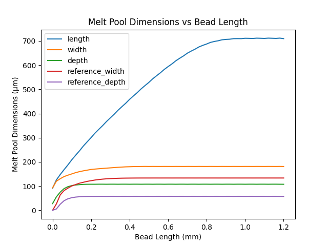
Plot melt pool statistics#
Obtain a Pandas DataFrame instance containing the melt pool
statistics by using the data_frame() method of the melt_pool
attribute of the summary object. The column names for the DataFrame
instance are described in the documentation for data_frame(). Use the
plot() method to plot the melt pool dimensions as a function
of bead length.
df = summary.melt_pool.data_frame().multiply(1e6)  # convert from meters to microns
df.index *= 1e3  # convert bead length from meters to millimeters

df.plot(
    y=[
        MeltPoolColumnNames.LENGTH,
        MeltPoolColumnNames.WIDTH,
        MeltPoolColumnNames.DEPTH,
        MeltPoolColumnNames.REFERENCE_WIDTH,
        MeltPoolColumnNames.REFERENCE_DEPTH,
    ],
    ylabel="Melt Pool Dimensions (µm)",
    xlabel="Bead Length (mm)",
    title="Melt Pool Dimensions vs Bead Length",
)
plt.show()

List melt pool statistics#
You can show a table of the melt pool statistics by typing the name of the
data frame object and pressing enter. For brevity, the following code
uses the head() method so that only the first few rows are shown.
Note, if running this example as a Python script, no output is shown.
df.head()
Save melt pool statistics#
Save the melt pool statistics to a CSV file using the
to_csv() method.
df.to_csv("melt_pool.csv")
Total running time of the script: (0 minutes 27.865 seconds)
